Switching between space and time: Spatio-temporal analysis with
cubble

Sherry Zhang

2022-09-27

Hi!

• A 3rd year PhD student in the Department of Econometrics and Business Statistics, Monash University

• My research centers on exploring multivariate spatio-temporal data with data wrangling and visualisation tool.

Roadmap

• Follow along with the slides at https://sherryzhang-rladiesmelb2022.netlify.app

• Go to the slide repo to run the code in the index.R yourself

After some introduction, I will first talk about spatial data with the sf package and then temporal data with the tsibble package before

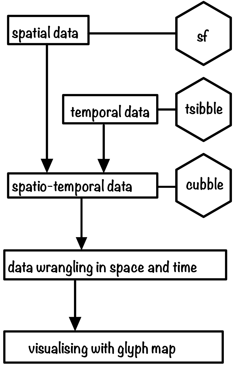
Spatio-temporal data

People can talk about a whole range of differnt things when they only refer to their data as spatio-temporal!

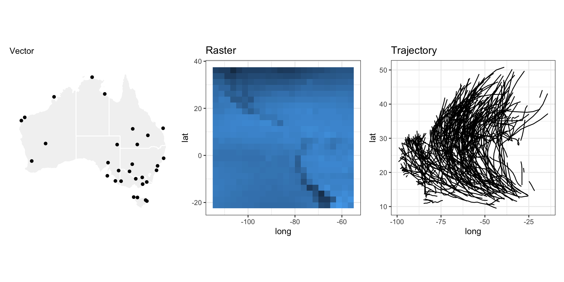
The focus of today will be on vector data

Data with different spatial and temporal characteristics can all sit under the big umbrella of spatio-temporal data.

Here we have three different types: vector, raster, trajectory data (explain each)

vector data have time series measured at a collection of locations

raster data use gridded cells to represent a continuous space and each cell has variables measured at different time point. You can think of it as take snapshots of space at various time points and stack them on top of each other

trajectory data, on the other hand, have points moving in the space and time in the same time. Here each point on these line would have a different long, lat and time marker.

These are three different representation of spatio-temporal data and they have their own tools for wrangling and visualisation

That’s why I always feel

Examples of vector data

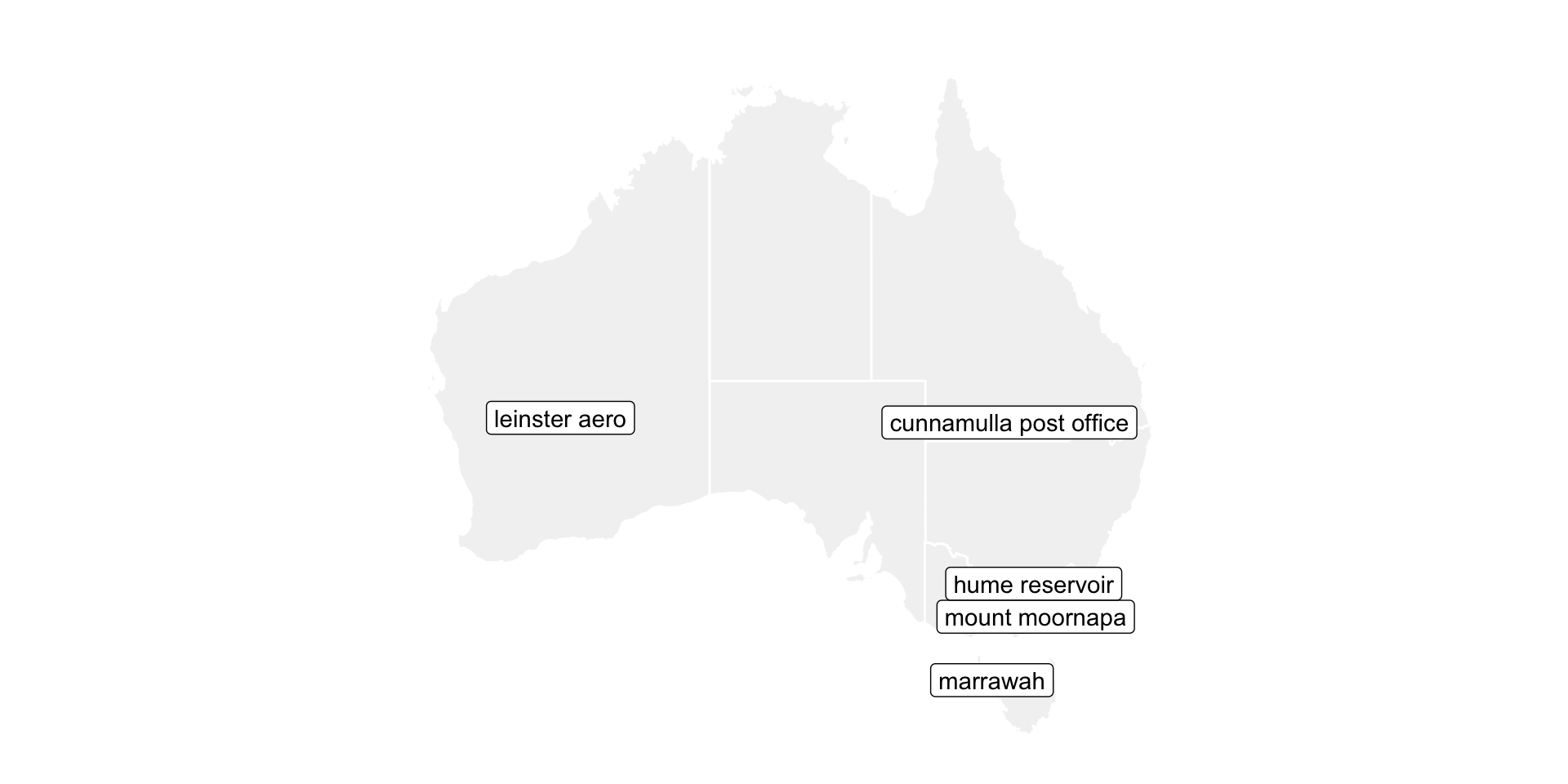
Physical sensors that measure the temperature, rainfall, wind speed & direction, water level, etc

A major source of vector spatio-temporal data is physical sensors that measures a range of climate variables

With these data, typically you will get the spatial data by choosing a list of stations of your interest and then query the temporal data.

Now we will first talk about the spatial component before moving to the temporal component.

Represent spatial data in R?

• A pair of longitude/ latitude (stations_dt)

# A tibble: 30 × 6
  id           long   lat  elev name                       wmo_id
  <chr>       <dbl> <dbl> <dbl> <chr>                       <dbl>
1 ASN00060139  153. -31.4   4.2 port macquarie airport aws  94786
2 ASN00068228  151. -34.4  10   bellambi aws                94749
# … with 28 more rows

• Simple features with sf (stations_sf)

Simple feature collection with 30 features and 4 fields
Geometry type: POINT
Dimension:     XY
Bounding box:  xmin: 114.0967 ymin: -41.8739 xmax: 152.8655 ymax: -11.6502
Geodetic CRS:  GDA94
# A tibble: 30 × 5
  id           elev name                       wmo_id            geometry
  <chr>       <dbl> <chr>                       <dbl>         <POINT [°]>
1 ASN00060139   4.2 port macquarie airport aws  94786 (152.8655 -31.4336)
2 ASN00068228  10   bellambi aws                94749 (150.9291 -34.3691)
# … with 28 more rows

There are two ways you can represent spatial data in R.

The first is to use two separate longitude and latitude columns

Another way is to use the simple feature representation with the sf package.

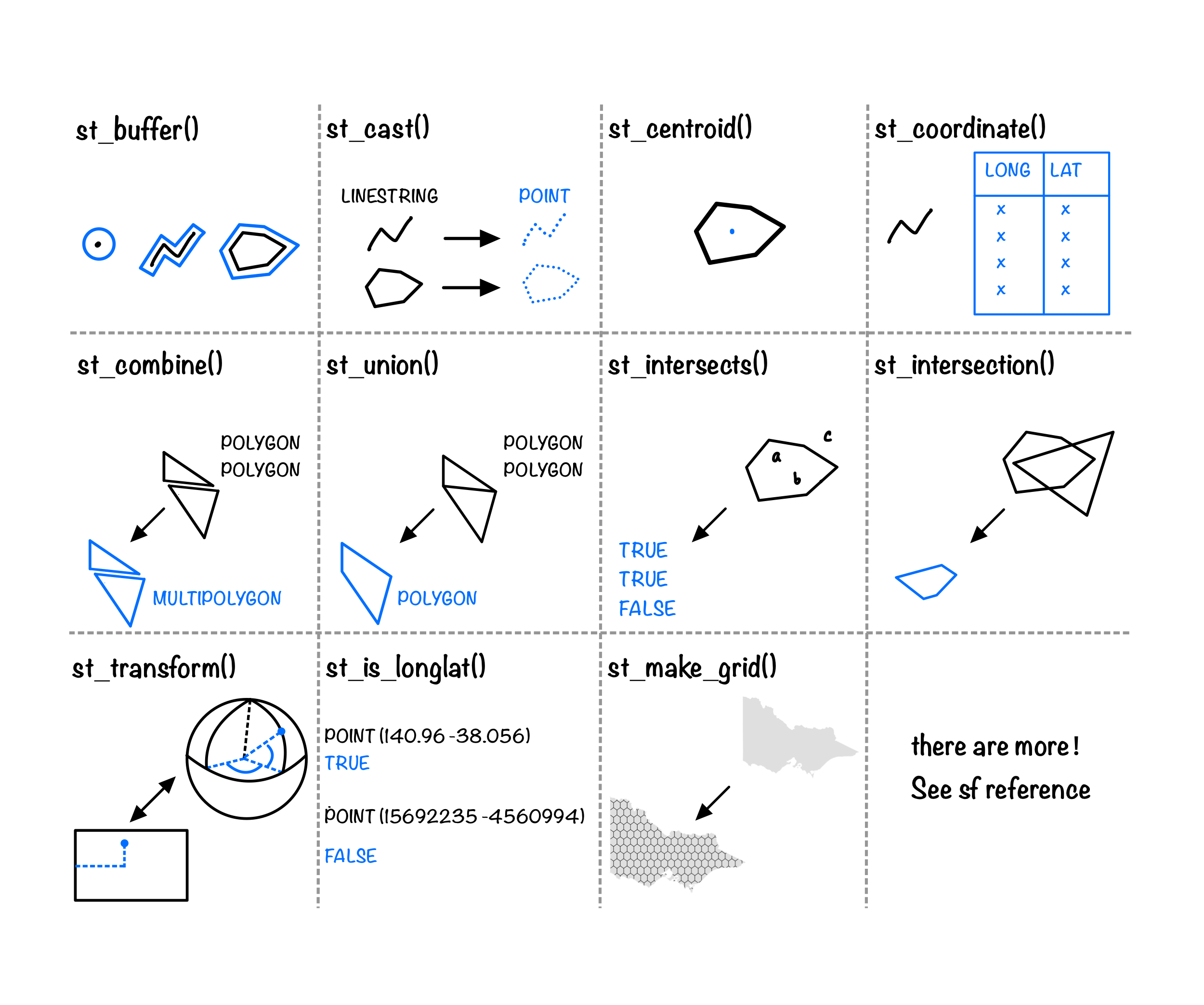
Geometrical operations with sf

The benefit of using the sf package is that the package also give you access to many geometrical operations.

Here I have a few examples ..

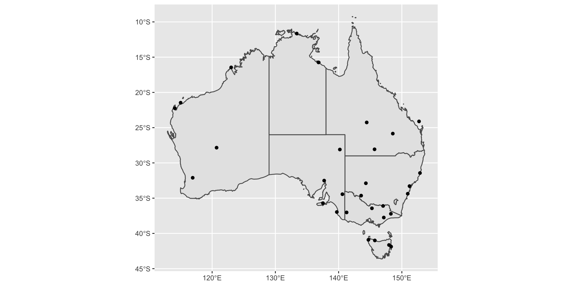
Ploting an sf object

ggplot() + 
  geom_sf(data = oz_simp) + 
  geom_sf(data = stations_sf)

set.seed(1234)
dt_lbl <- stations_sf %>% arrange(id) %>% sample_n(5)
ggplot() +
  geom_sf(
    data = oz_simp, 
    fill = "grey95", color = "white") +
  geom_sf_label(
    data = dt_lbl, 
    aes(label = name)) + 
  ggthemes::theme_map() 

Also the geom_sf function allow you to supply an sf object and will automatically plot the geometry

The goem_sf_label allows you to put the label on the points and there are themes and aesthetics you can use to make the map pretty.

Look into an sf object - POINTS

dt # simple feature (sf)

Simple feature collection with 2 features and 6 fields
Geometry type: POINT
Dimension:     XY
Bounding box:  xmin: 150.9291 ymin: -34.3691 xmax: 152.8655 ymax: -31.4336
Geodetic CRS:  GDA94
# A tibble: 2 × 7
  id            lat  long  elev name            wmo_id            geometry
  <chr>       <dbl> <dbl> <dbl> <chr>            <dbl>         <POINT [°]>
1 ASN00060139 -31.4  153.   4.2 port macquarie…  94786 (152.8655 -31.4336)
2 ASN00068228 -34.4  151.  10   bellambi aws     94749 (150.9291 -34.3691)

(pnt_sfc <- dt$geometry) # simple feature column (sfc)

Geometry set for 2 features 
Geometry type: POINT
Dimension:     XY
Bounding box:  xmin: 150.9291 ymin: -34.3691 xmax: 152.8655 ymax: -31.4336
Geodetic CRS:  GDA94
POINT (152.8655 -31.4336)
POINT (150.9291 -34.3691)

(pnt_sfg <- pnt_sfc[[1]]) # simple feature geometry (sfg) - POINT

POINT (152.8655 -31.4336)

For beginners, the sf header and the geometry representation could be difficult to work with

Here are three common prints you may see

explain what you can read here

It may seem confusing as how can you perform operations on these objects, especially the sfc and the sfg. What is underneath these prints? I will now show you that these representations can all be boiled down to the basic structure you’re already familiar with

Look into an sf object - POINTS (2)

The point sfg is a paired vector with special class labels

pnt_sfg # simple feature geometry (sfg) - POINTS

POINT (152.8655 -31.4336)

typeof(pnt_sfg) 

[1] "double"

attributes(pnt_sfg)

$class
[1] "XY"    "POINT" "sfg"  

unclass(pnt_sfg)

[1] 152.8655 -31.4336

The POINT (152.8655 -31.4336) format is called well-known text, which is a human-readable encoding used by sf

Look into an sf object - POINTS (3)

The sfc is a list of sfg with special attributes

pnt_sfc # simple feature column (sfc)

Geometry set for 1 feature 
Geometry type: POINT
Dimension:     XY
Bounding box:  xmin: 152.8655 ymin: -31.4336 xmax: 152.8655 ymax: -31.4336
Geodetic CRS:  GDA94
POINT (152.8655 -31.4336)
POINT (150.9291 -34.3691)

typeof(pnt_sfc)

[1] "list"

names(attributes(pnt_sfc))

[1] "class"     "precision" "bbox"      "crs"       "n_empty"  

unclass(pnt_sfc)[1:2]

[[1]]
POINT (152.8655 -31.4336)

[[2]]
POINT (150.9291 -34.3691)

Other geoms (1/3) - LINESTRING

The linestring sfg is a matrix of paired doubles

(ls_sfg <- ls_sfc[[1]])

LINESTRING (149.2317 -35.222, 149.2716 -35.2708, 149.3153 -35.27623, 149.3972 -35.32425, 149.3363 -35.33988, 149.2493 -35.33013, 149.2045 -35.34761, 149.1464 -35.4153, 149.1352, ...)

typeof(ls_sfg)

[1] "double"

unclass(ls_sfg)

          [,1]      [,2]
 [1,] 149.2317 -35.22200
 [2,] 149.2716 -35.27080
 [3,] 149.3153 -35.27623
 [4,] 149.3972 -35.32425
 [5,] 149.3363 -35.33988
 [6,] 149.2493 -35.33013
 [7,] 149.2045 -35.34761
 [8,] 149.1464 -35.41530
 [9,] 149.1352 -35.45369
[10,] 149.1516 -35.49320
[11,] 149.1325 -35.54950
[12,] 149.1405 -35.58829
[13,] 149.0781 -35.58642
[14,] 149.0950 -35.67682
[15,] 149.1094 -35.69659
[16,] 149.0907 -35.76562
[17,] 149.1011 -35.80506
[18,] 149.0488 -35.92041
[19,] 149.0122 -35.89970
[20,] 148.9584 -35.89179
[21,] 148.9127 -35.85546
[22,] 148.8894 -35.72272
[23,] 148.8347 -35.74051
[24,] 148.7884 -35.69781
[25,] 148.7985 -35.66698
[26,] 148.7689 -35.60426
[27,] 148.7628 -35.49550
[28,] 148.7858 -35.40891
[29,] 148.8087 -35.38246
[30,] 148.7935 -35.33912
[31,] 148.8101 -35.30745
[32,] 149.1209 -35.12442
[33,] 149.1891 -35.16552
[34,] 149.1903 -35.19435
[35,] 149.2317 -35.22200

Other geoms (2/3) - POLYGONS

POLYGON sfg is a list where each element is a matrix of paired vectors

(pol_sfg <- pol_sfc[[1]])

POLYGON ((149.2317 -35.222, 149.2716 -35.2708, 149.3153 -35.27623, 149.3972 -35.32425, 149.3363 -35.33988, 149.2493 -35.33013, ...))

typeof(pol_sfg)

[1] "list"

unclass(pol_sfg)

[[1]]
          [,1]      [,2]
 [1,] 149.2317 -35.22200
 [2,] 149.2716 -35.27080
 [3,] 149.3153 -35.27623
 [4,] 149.3972 -35.32425
 [5,] 149.3363 -35.33988
 [6,] 149.2493 -35.33013
 [7,] 149.2045 -35.34761
 [8,] 149.1464 -35.41530
 [9,] 149.1352 -35.45369
[10,] 149.1516 -35.49320
[11,] 149.1325 -35.54950
[12,] 149.1405 -35.58829
[13,] 149.0781 -35.58642
[14,] 149.0950 -35.67682
[15,] 149.1094 -35.69659
[16,] 149.0907 -35.76562
[17,] 149.1011 -35.80506
[18,] 149.0488 -35.92041
[19,] 149.0122 -35.89970
[20,] 148.9584 -35.89179
[21,] 148.9127 -35.85546
[22,] 148.8894 -35.72272
[23,] 148.8347 -35.74051
[24,] 148.7884 -35.69781
[25,] 148.7985 -35.66698
[26,] 148.7689 -35.60426
[27,] 148.7628 -35.49550
[28,] 148.7858 -35.40891
[29,] 148.8087 -35.38246
[30,] 148.7935 -35.33912
[31,] 148.8101 -35.30745
[32,] 149.1209 -35.12442
[33,] 149.1891 -35.16552
[34,] 149.1903 -35.19435
[35,] 149.2317 -35.22200

And lastly … MULTIPOLYGONS!

MULTIPOLYGON sfg is a nested list where each list element can contain multiple matrices of paired vectors

(mpol_sfg <- mpol_sfc[[1]])

MULTIPOLYGON (((145.2859 -38.3962, 145.2903 -38.28367, 145.4109 -38.37078, 145.2859 -38.3962)), ((140.9657 -38.05599, 140.9739 -37.46209, 140.9693 -36.79305, 140.9631 -35.74853, 140.9656 -35.00826, 140.9617 -34.09582, ...)))

typeof(mpol_sfg)

[1] "list"

length(unclass(mpol_sfg))

[1] 2

unclass(mpol_sfg)

[[1]]
[[1]][[1]]
         [,1]      [,2]
[1,] 145.2859 -38.39620
[2,] 145.2903 -38.28367
[3,] 145.4109 -38.37078
[4,] 145.2859 -38.39620


[[2]]
[[2]][[1]]
           [,1]      [,2]
  [1,] 140.9657 -38.05599
  [2,] 140.9739 -37.46209
  [3,] 140.9693 -36.79305
  [4,] 140.9631 -35.74853
  [5,] 140.9656 -35.00826
  [6,] 140.9617 -34.09582
  [7,] 141.0089 -34.04466
  [8,] 141.2610 -34.07898
  [9,] 141.3576 -34.11069
 [10,] 141.5176 -34.20645
 [11,] 141.7049 -34.09569
 [12,] 141.8424 -34.13253
 [13,] 141.8991 -34.11149
 [14,] 142.0745 -34.13049
 [15,] 142.0821 -34.17299
 [16,] 142.2203 -34.18167
 [17,] 142.2385 -34.30782
 [18,] 142.3337 -34.33930
 [19,] 142.3684 -34.52709
 [20,] 142.4347 -34.57615
 [21,] 142.5262 -34.75981
 [22,] 142.6968 -34.72016
 [23,] 142.6995 -34.60315
 [24,] 142.7635 -34.59674
 [25,] 143.0400 -34.70251
 [26,] 143.1041 -34.69400
 [27,] 143.3515 -34.79600
 [28,] 143.3196 -34.96870
 [29,] 143.3470 -35.10478
 [30,] 143.3964 -35.19311
 [31,] 143.5639 -35.20263
 [32,] 143.5637 -35.31612
 [33,] 143.6423 -35.40104
 [34,] 143.7465 -35.38860
 [35,] 143.8666 -35.48032
 [36,] 144.0479 -35.55617
 [37,] 144.1175 -35.62593
 [38,] 144.3757 -35.80121
 [39,] 144.4082 -35.90422
 [40,] 144.5833 -36.03903
 [41,] 144.8058 -36.12384
 [42,] 144.9236 -35.98895
 [43,] 144.9750 -35.88343
 [44,] 145.0729 -35.82776
 [45,] 145.2465 -35.83041
 [46,] 145.3524 -35.86580
 [47,] 145.5340 -35.80529
 [48,] 145.6847 -35.93075
 [49,] 145.7934 -35.98282
 [50,] 145.9080 -35.95356
 [51,] 145.9891 -36.01308
 [52,] 146.2618 -36.01580
 [53,] 146.3877 -36.03527
 [54,] 146.4143 -35.97545
 [55,] 146.5179 -35.96006
 [56,] 146.6870 -36.04082
 [57,] 146.8363 -36.08219
 [58,] 147.0162 -36.08950
 [59,] 147.1372 -36.02862
 [60,] 147.2043 -36.04989
 [61,] 147.3522 -36.03229
 [62,] 147.4043 -35.94356
 [63,] 147.4986 -35.94664
 [64,] 147.5552 -36.00321
 [65,] 147.7084 -35.92854
 [66,] 147.9140 -35.99795
 [67,] 147.9976 -36.04777
 [68,] 148.0289 -36.14008
 [69,] 148.0383 -36.36556
 [70,] 148.1247 -36.46484
 [71,] 148.1244 -36.55098
 [72,] 148.2174 -36.59885
 [73,] 148.1851 -36.69222
 [74,] 148.1949 -36.79625
 [75,] 149.1998 -37.20119
 [76,] 149.9763 -37.50503
 [77,] 149.7393 -37.58451
 [78,] 149.6747 -37.68584
 [79,] 149.4948 -37.76847
 [80,] 149.2516 -37.78179
 [81,] 148.8087 -37.78642
 [82,] 148.6260 -37.80814
 [83,] 148.3662 -37.80395
 [84,] 148.1792 -37.83164
 [85,] 147.7884 -37.95525
 [86,] 147.4672 -38.15915
 [87,] 147.0672 -38.47512
 [88,] 146.9320 -38.59602
 [89,] 146.7857 -38.64632
 [90,] 146.4438 -38.69492
 [91,] 146.2675 -38.68791
 [92,] 146.1856 -38.74344
 [93,] 146.2656 -38.80531
 [94,] 146.2919 -38.90428
 [95,] 146.4170 -38.84892
 [96,] 146.4873 -38.90615
 [97,] 146.4367 -38.97907
 [98,] 146.4209 -39.12585
 [99,] 146.2739 -38.99612
[100,] 146.1842 -38.86951
[101,] 146.0632 -38.81177
[102,] 145.9189 -38.90688
[103,] 145.8715 -38.77944
[104,] 145.7308 -38.64813
[105,] 145.5647 -38.65419
[106,] 145.4237 -38.53648
[107,] 145.4329 -38.42871
[108,] 145.5525 -38.35457
[109,] 145.4883 -38.23615
[110,] 145.3442 -38.21445
[111,] 145.2550 -38.23743
[112,] 145.1299 -38.39045
[113,] 145.0257 -38.47967
[114,] 144.9244 -38.49740
[115,] 144.8369 -38.37040
[116,] 144.9750 -38.32697
[117,] 145.1213 -38.13339
[118,] 145.0906 -38.01495
[119,] 145.0307 -37.99351
[120,] 144.9638 -37.85576
[121,] 144.8085 -37.88033
[122,] 144.6502 -38.00202
[123,] 144.4874 -38.07828
[124,] 144.3979 -38.07382
[125,] 144.3561 -38.13840
[126,] 144.4807 -38.16449
[127,] 144.6318 -38.10734
[128,] 144.7197 -38.14612
[129,] 144.6142 -38.29214
[130,] 144.4357 -38.28130
[131,] 144.2516 -38.38841
[132,] 144.0365 -38.47578
[133,] 143.9731 -38.56636
[134,] 143.8421 -38.67908
[135,] 143.6854 -38.73536
[136,] 143.5557 -38.85494
[137,] 143.3569 -38.75435
[138,] 143.2203 -38.76029
[139,] 143.0217 -38.62625
[140,] 142.8611 -38.60563
[141,] 142.5633 -38.42200
[142,] 142.3722 -38.34942
[143,] 142.1482 -38.38969
[144,] 141.8849 -38.26629
[145,] 141.7420 -38.25311
[146,] 141.5992 -38.32107
[147,] 141.5575 -38.42235
[148,] 141.4067 -38.36934
[149,] 141.3574 -38.27460
[150,] 141.2278 -38.17065
[151,] 140.9657 -38.05599

Geometry types - summary

• The sf, sfc, and sfg objects have informative header prints but they can be boiled down to basic data structures that we’re already familiar with

• There are more than just introduced geometry types: MULTIPOINTS, MULTILINESTRING, etc

• In practice, you don’t have to decompose/ manipulate these vectors or matrices manually, existing geometrical operations (st_*()) and visualisation tools (geom_sf()) will do that for you.

Geometrical operations with sf again

Aggregate time series with tsibble

Time series of weather station data

ts %>% 
  ggplot(aes(x = date, y = tmax, group = id)) + 
  geom_line(alpha = 0.6) + 
  theme_bw()

For the 30 stations I have shown you before, we also have daily information on precipitation, maximum and minimum temperature.

Here I plot the maximum temperature of each station in 2020 and because it is daily data, these lines are quite wiggly.

How’s the data quality from BOM?

First cast the data into a tsibble, before using tsibble::count_gaps() for data quality check

ts

# A tibble: 10,632 × 5
   id          date        prcp  tmax  tmin
   <chr>       <date>     <dbl> <dbl> <dbl>
 1 ASN00003057 2020-01-01     0  36.7  26.9
 2 ASN00003057 2020-01-02    41  34.2  24  
 3 ASN00003057 2020-01-03     0  35    25.4
 4 ASN00003057 2020-01-04    40  29.1  25.4
 5 ASN00003057 2020-01-05  1640  27.3  24.3
 6 ASN00003057 2020-01-06  1832  29.2  23.2
 7 ASN00003057 2020-01-07    42  36    21  
 8 ASN00003057 2020-01-08   300  31.5  25  
 9 ASN00003057 2020-01-09    90  32.2  25.3
10 ASN00003057 2020-01-10     0  34    25.9
# … with 10,622 more rows

library(tsibble)
(ts_tsibble <- ts %>% 
   as_tsibble(key = id, index = date))

# A tsibble: 10,632 x 5 [1D]
# Key:       id [30]
   id          date        prcp  tmax  tmin
   <chr>       <date>     <dbl> <dbl> <dbl>
 1 ASN00003057 2020-01-01     0  36.7  26.9
 2 ASN00003057 2020-01-02    41  34.2  24  
 3 ASN00003057 2020-01-03     0  35    25.4
 4 ASN00003057 2020-01-04    40  29.1  25.4
 5 ASN00003057 2020-01-05  1640  27.3  24.3
 6 ASN00003057 2020-01-06  1832  29.2  23.2
 7 ASN00003057 2020-01-07    42  36    21  
 8 ASN00003057 2020-01-08   300  31.5  25  
 9 ASN00003057 2020-01-09    90  32.2  25.3
10 ASN00003057 2020-01-10     0  34    25.9
# … with 10,622 more rows

The data are downloaded from the Bureau of Meteorology and are structued in a long table

[introduce data]

We would like to know about the data quatlity before proceed to any analysis and the tsibble package has a function count_gaps() for that.

The count_gaps() function requires the data to be a tsibble object, so we first need to create a tsibble from our data.

[explain creation]

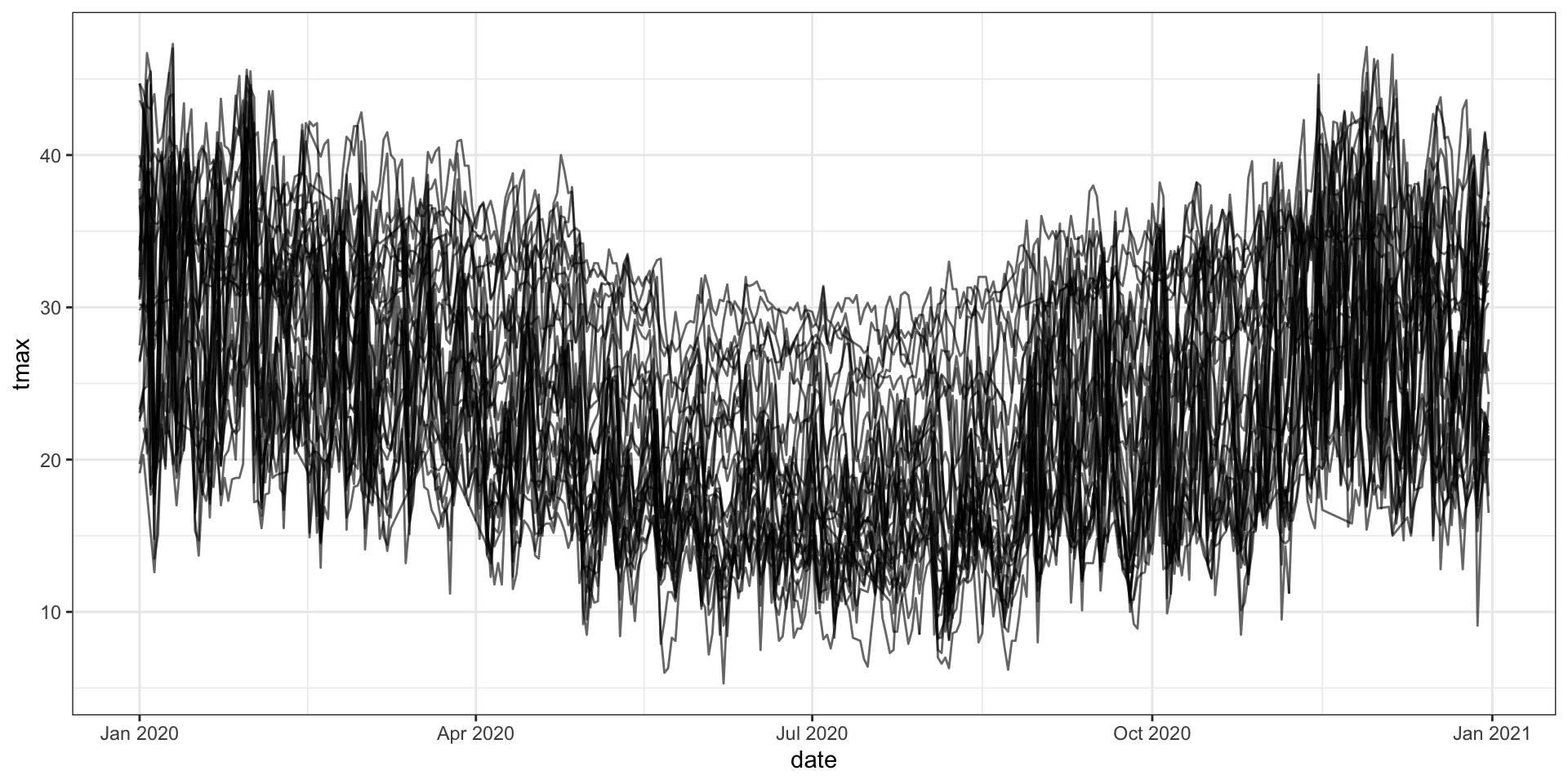
How’s the data quality from BOM?

(missings <- ts_tsibble %>% tsibble::count_gaps())

# A tibble: 112 × 4
  id          .from      .to           .n
  <chr>       <date>     <date>     <int>
1 ASN00003057 2020-02-17 2020-02-18     2
2 ASN00003057 2020-02-25 2020-03-01     6
3 ASN00003057 2020-03-07 2020-03-09     3
4 ASN00003057 2020-03-11 2020-03-13     3
5 ASN00003057 2020-03-25 2020-03-27     3
# … with 107 more rows

missings <- missings %>% group_by(id) %>% mutate(ttl_n = sum(.n))
missings %>% 
  ggplot() + 
  geom_errorbar(aes(xmin = .from, xmax = .to, y = fct_reorder(id, ttl_n)), 
                width = 0.2) + 
  theme_bw() + 
  scale_x_date(date_breaks = "1 month", date_labels = "%b") + 
  ylab("Station ID")

Then we can pipe the created tsibble into count_gaps and the output of it is a separate table summary

Here the first chunk of missing is for station 3057, from 02-17 to 02-18, for two days

We can plot these missing gaps with geom errorbar.

In this code, I order the stations from the one has the most total missing to the least

How’s the data quality from BOM?

Despite some small missingness for a day or two here and there, overall, these stations don’t have a long period of missing.

The only few that we may need to be cautious are …

Bear in mind that not all of the stations are automatic, someone needs to go to the station everyday 9 am to write down these numbers, so this amount of missingness is acceptable to me

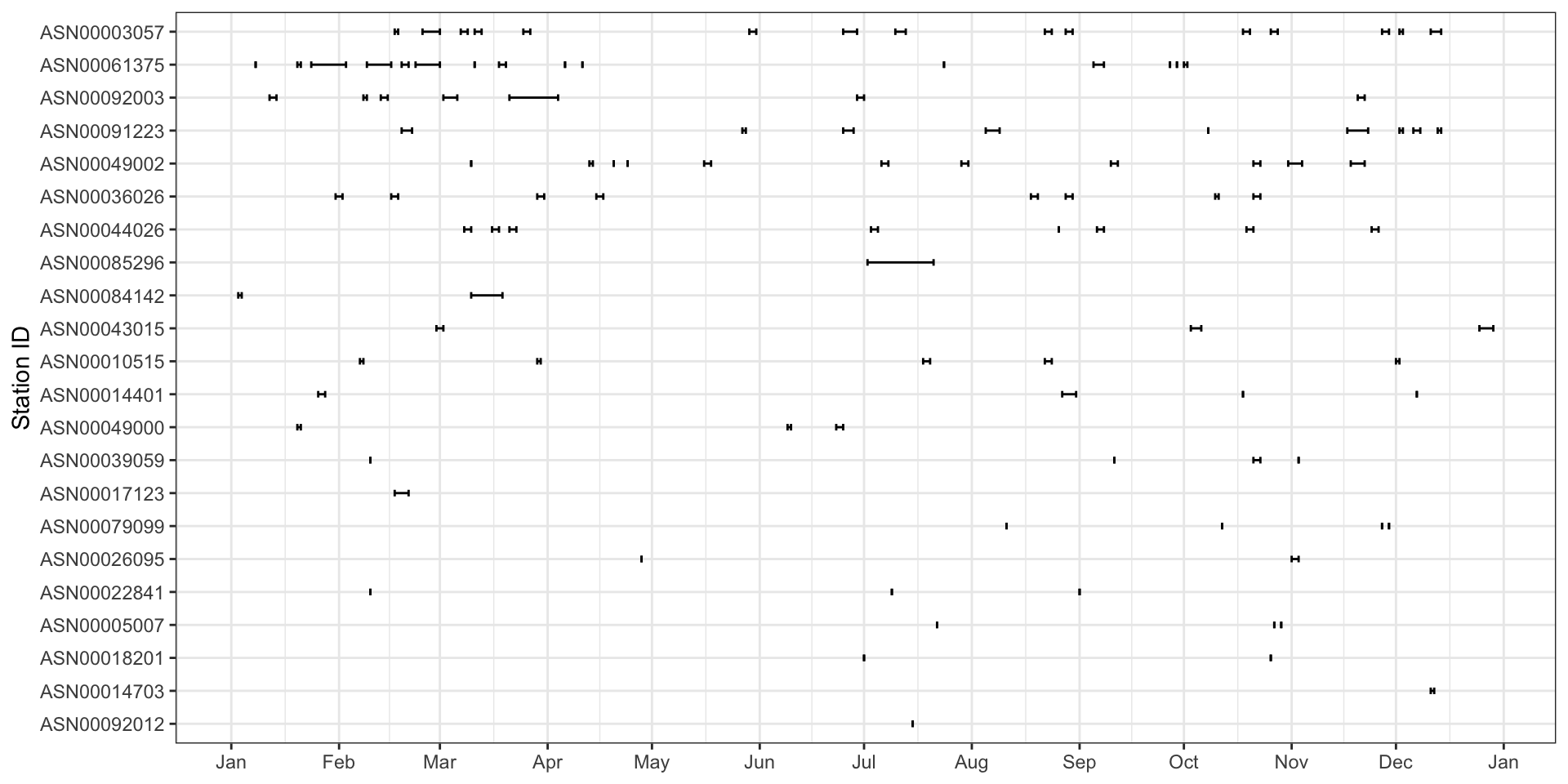
Make the inexplicit NAs explicit

single <- ts_tsibble %>% 
  filter(id == "ASN00003057")
single_filled <- single %>% 
  tsibble::fill_gaps()

single %>% 
  filter(date >= "2020-02-15") 

# A tsibble: 271 x 5 [1D]
# Key:       id [1]
  id          date        prcp  tmax  tmin
  <chr>       <date>     <dbl> <dbl> <dbl>
1 ASN00003057 2020-02-15     0  33.7  25.5
2 ASN00003057 2020-02-16     0  33.5  28.5
3 ASN00003057 2020-02-19    20  34    24.4
4 ASN00003057 2020-02-20     0  34.1  26.5
5 ASN00003057 2020-02-21     0  34.5  25.7
# … with 266 more rows

single_filled %>% 
  filter(date >= "2020-02-15")

# A tsibble: 321 x 5 [1D]
# Key:       id [1]
  id          date        prcp  tmax  tmin
  <chr>       <date>     <dbl> <dbl> <dbl>
1 ASN00003057 2020-02-15     0  33.7  25.5
2 ASN00003057 2020-02-16     0  33.5  28.5
3 ASN00003057 2020-02-17    NA  NA    NA  
4 ASN00003057 2020-02-18    NA  NA    NA  
5 ASN00003057 2020-02-19    20  34    24.4
# … with 316 more rows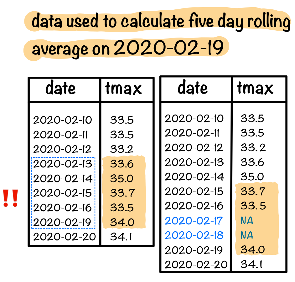

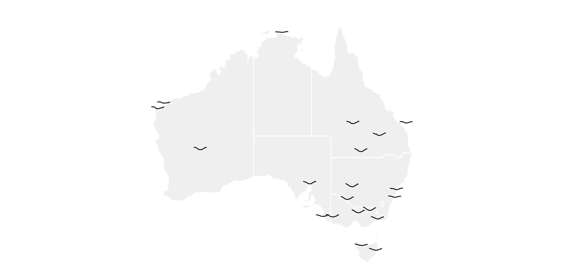
Sometimes, the missingness is not explicitly stated

We can inspect to see there is a jump from teh 16th to the 19th but the data do not speak for itself.

These inexplicit NAs can bring in some unexpected error in your calculation that you’re not even aware of. For example,

Without explicitly register the two missing dates, we will calculating using the four rows directly above the 19th of Feb and here it will be from 13th to 16th.

while if the missingness is properly registered, we will be using the correct dates on the calculation.

The fill_gaps() functions from the tsibble package can populate the time into a complete grid and register the missing cells with NAs

Space and time at the same time with cubble

Goal of today: glyph map

One of today’s goals is for everyone to make a glyph map similar to this by the end of the session.

We need a data structure to manpulate the data in space and in time, the data manipulation part.

We also need a way to draw the small multiples on the map, the visualisation part.

Cubble - a spatio-temporal vector data structure

For the wrangling part, I will use the cubble package

A cubble has two forms, a nested form where all the temporal data is nested in a list column, just as how the geometry is a list column in the sf package.

This form can be used for calculation on the space or make per station summary from the time series

Another form is called the long form, which will elaborate the time series data in the long form and temporaily hide the spatial data.

With the long form, you can make some temporal summary of the data.

Here the illustration shows you how to turn a nested cubble into the long form with face_temporal() and backward with face_spatial().

Cast your data into a cubble

(cb <- as_cubble(
  list(spatial = stations_sf, temporal = ts),
  key = id, index = date, coords = c(long, lat)
))

# cubble:   id [30]: nested form [sf]
# bbox:     [114.09, -41.88, 152.87, -11.65]
# temporal: date [date], prcp [dbl], tmax [dbl], tmin [dbl]
  id            lat  long  elev name   wmo_id            geometry ts      
  <chr>       <dbl> <dbl> <dbl> <chr>   <dbl>         <POINT [°]> <list>  
1 ASN00003057 -16.5  123.   7   cygne…  94201 (123.0086 -16.4514) <tibble>
2 ASN00005007 -22.2  114.   5   learm…  94302 (114.0967 -22.2406) <tibble>
3 ASN00005084 -21.5  115.   5   theve…  94303 (115.0197 -21.4606) <tibble>
4 ASN00010515 -32.1  117. 199   bever…  95615 (116.9247 -32.1083) <tibble>
5 ASN00012314 -27.8  121. 497   leins…  95448 (120.7031 -27.8386) <tibble>
6 ASN00014401 -11.7  133.  19.2 warru…  94139 (133.3796 -11.6502) <tibble>
7 ASN00014703 -15.7  137.  12.2 centr…  94248 (136.8192 -15.7426) <tibble>
# … with 23 more rows

There are different ways you can create a cubble.

If you have the spatial and temporal data in two separate tables, you can supply them as a list.

Then you need to specify some parameters. The key and index are the same as how you would construct a tsibble

And cubble requires an additional coords parameter for coordinates.

This is how the created cubble looks like

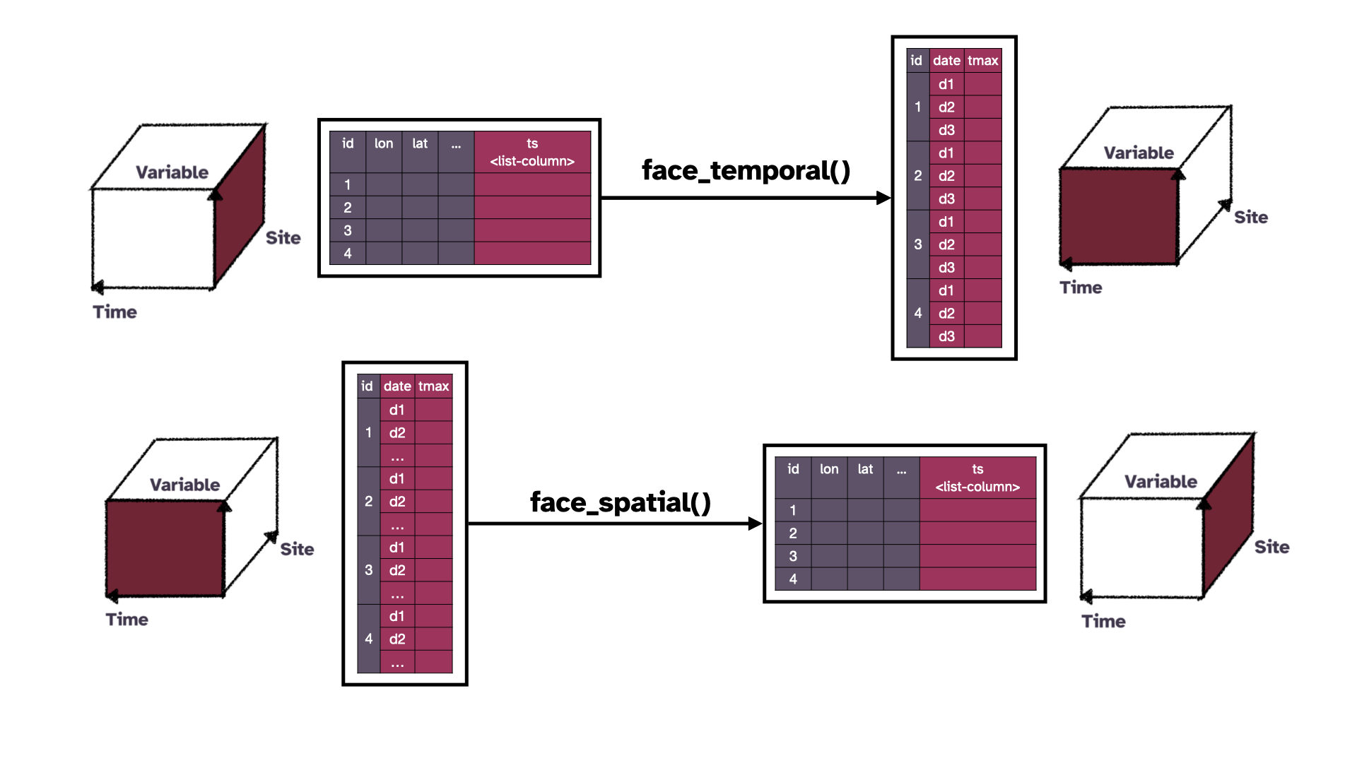
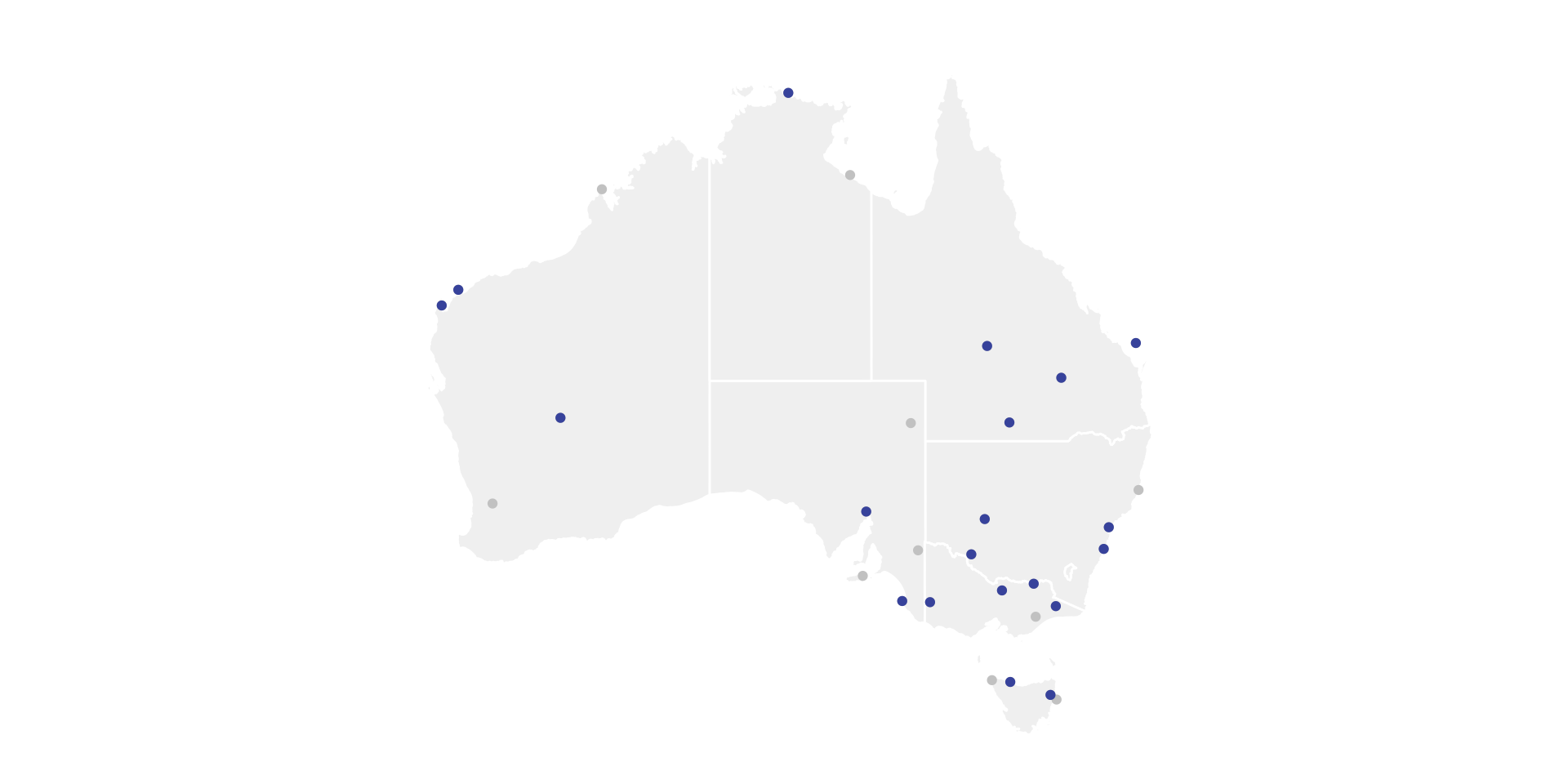
Subset on space

set.seed(0927)
cb_space <- cb %>% slice_sample(n = 20)

Summarise in time

(cb_tm <- cb_space %>% 
  face_temporal() %>% 
  group_by(month = lubridate::month(date)) %>% 
  summarise(tmax = mean(tmax, na.rm = TRUE))
  )

# cubble:  month, id [20]: long form
# bbox:    [114.09, -41.65, 152.72, -11.65]
# spatial: lat [dbl], long [dbl], elev [dbl], name [chr], wmo_id [dbl],
#   geometry [POINT [°]]
  id          month  tmax
  <chr>       <dbl> <dbl>
1 ASN00005007     1  38.8
2 ASN00005007     2  37.5
3 ASN00005007     3  38.1
4 ASN00005007     4  35.8
5 ASN00005007     5  28.6
6 ASN00005007     6  26.6
7 ASN00005007     7  27.4
# … with 233 more rows

Move coordinates into time

(cb_glyph <- cb_tm %>% unfold(long, lat))

# cubble:  month, id [20]: long form
# bbox:    [114.09, -41.65, 152.72, -11.65]
# spatial: lat [dbl], long [dbl], elev [dbl], name [chr], wmo_id [dbl],
#   geometry [POINT [°]]
  id          month  tmax  long   lat
  <chr>       <dbl> <dbl> <dbl> <dbl>
1 ASN00005007     1  38.8  114. -22.2
2 ASN00005007     2  37.5  114. -22.2
3 ASN00005007     3  38.1  114. -22.2
4 ASN00005007     4  35.8  114. -22.2
5 ASN00005007     5  28.6  114. -22.2
6 ASN00005007     6  26.6  114. -22.2
7 ASN00005007     7  27.4  114. -22.2
# … with 233 more rows

Now we have longitude and latitude in the nested form and monthly summarised tmax in the long form, the last thing we need to do is to move them into the same table before making the glyph map.

Here you need the verb unfold

Glyph map transformation

DATA %>% 
  ggplot() +
  geom_glyph(
    aes(x_major = X_MAJOR, x_minor = X_MINOR, 
        y_major = Y_MAJOR, y_minor = Y_MINOR)) + 
  ...

The glyphmap is essentially a transformation of temporal variable into space.

Here (1) shows a single station with its long and lat coordinate and (2) is its associated time series. We can use linear algebra to transform the temporal axes into the spatial scale as in (3) and once we have the time series in the transformed axes, they can be placed onto the map as in (4)

To make a glyph map, you can use the geom_glyph function from cubble.

It requires a pair of major and a pair of minor variable as aesthetics

The major variable are the spatial coordinates, long and lat here and hte minor variable are the temporal coordinates, date and tmax here.

Here (1) and (2) are

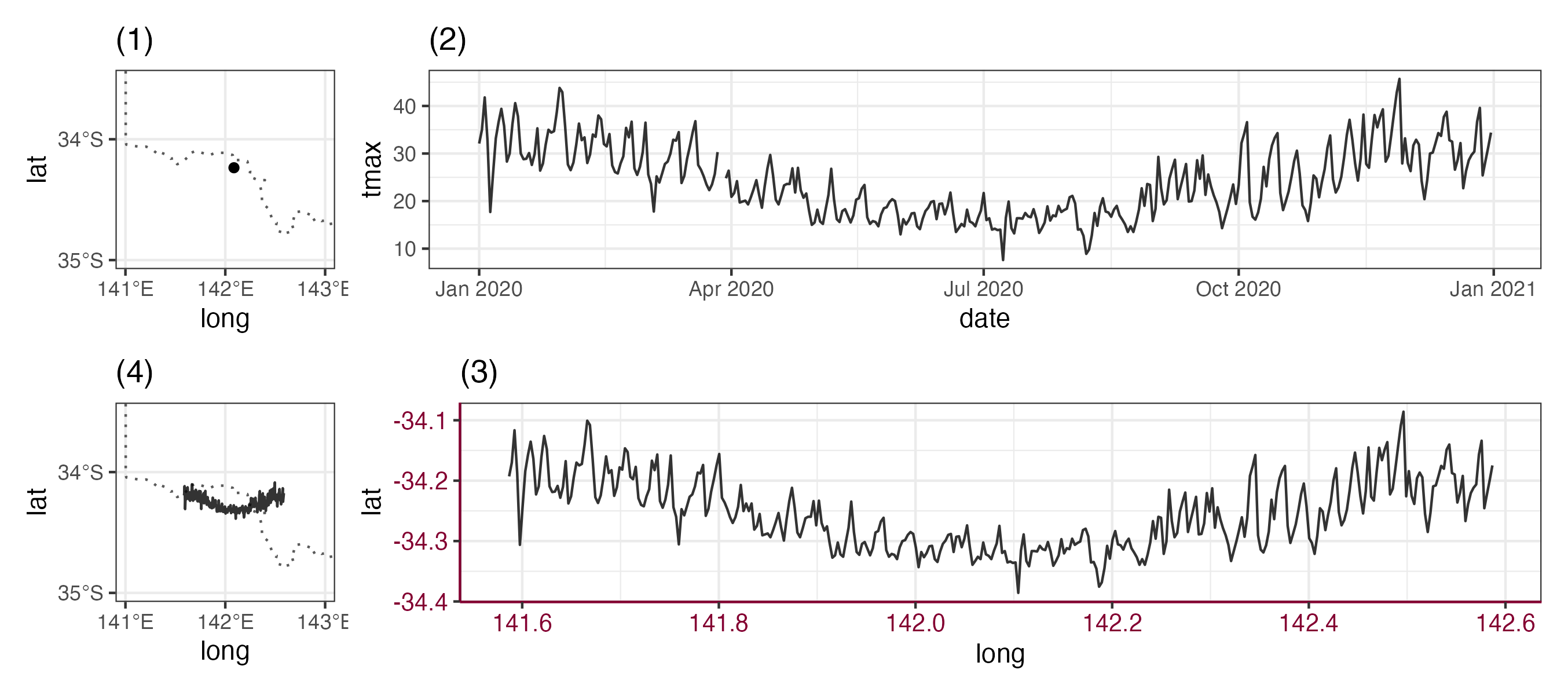
Making your first glyph map

Code

cb <- as_cubble(
  list(spatial = stations_sf, temporal = ts),
  key = id, index = date, coords = c(long, lat)
)
set.seed(0927)
cb_glyph <- cb %>% 
  slice_sample(n = 20) %>% 
  face_temporal() %>% 
  group_by(month = lubridate::month(date)) %>% 
  summarise(tmax = mean(tmax, na.rm = TRUE)) %>% 
  unfold(long, lat)
ggplot() + 
  geom_sf(data = oz_simp, fill = "grey95", color = "white") +
  geom_glyph(
    data = cb_glyph,
    aes(x_major = long, x_minor = month, y_major = lat, y_minor = tmax),
    width = 2, height = 0.7) + 
  ggthemes::theme_map()

Your Time

1. Create a cubble object from the spatial and temporal data given

2. Perform an operation on the space in the nested form

3. Switch to the long form to summarise the temporal data

4. Make a glyph map!

Further reading

• Spatial Data Science with application to R: https://r-spatial.org/book/
• sf: https://r-spatial.github.io/sf/index.html
• tsibble: https://tsibble.tidyverts.org/
• cubble: https://huizezhang-sherry.github.io/cubble/

Acknowledgements

• The slides are made with Quarto

• All the materials used to prepare the slides are available at sherryzhang-RLadiesMelb2022.netlify.app